Neural Network

Neural networks rely on two key mathematical processes: forward propagation (for predictions) and backward propagation (for learning via gradient descent).

The Math Behind Neural Network Forward and Backward Propagation

Neural networks rely on two key mathematical processes: forward propagation (for predictions) and backward propagation (for learning via gradient descent). In this post, we break down the core math behind these steps using a simple 3-layer neural network example. Hand-written calculations and diagrams from my notes are included for clarity.

---

Network Architecture

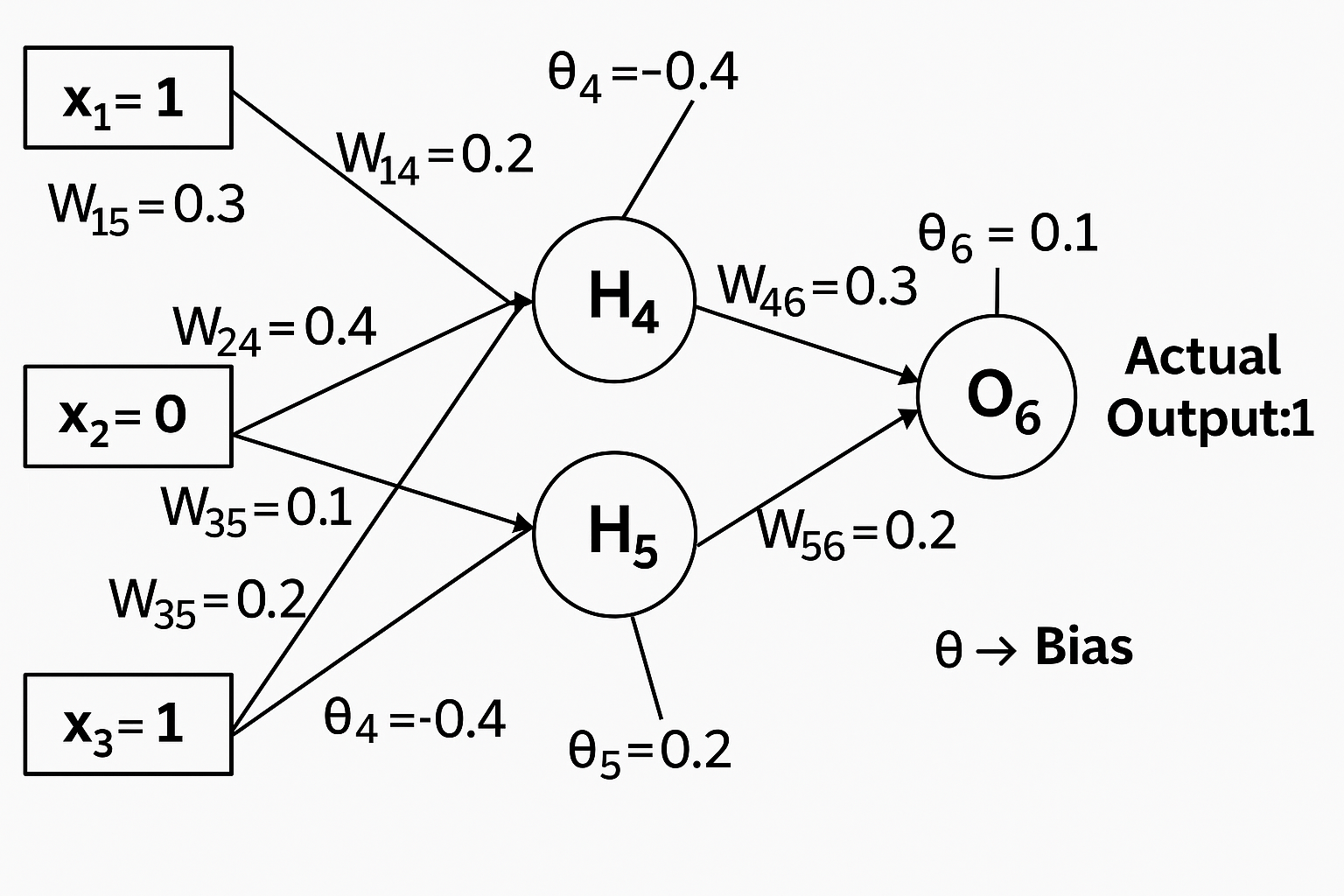
We consider a neural network with:

• Input layer: 3 neurons (x₁, x₂, x₃)
• Hidden layer: 2 neurons (h₄, h₅)
• Output layer: 1 neuron (o₆)

Input Layer (x₁, x₂, x₃) → Hidden Layer (h₄, h₅) → Output Layer (o₆)

---

1. Forward Pass

The forward pass computes the output of each neuron layer-by-layer using weights (ω), biases (b), and activation functions (sigmoid here).

Hidden Layer Calculations

For neuron 4 (h₄):

a4 = sigmoid(inputs * weights + b4)

From the notes:

a4 = 1 / (1 + exp(-(-0.7))) = 0.332

For neuron 5 (h₅):

a5 = 1 / (1 + exp(-0.1)) = 0.325

Output Layer Calculation

o6 = sigmoid(a4 * ω46 + a5 * ω56 + b6)

a6 = 1 / (1 + exp(-(-0.206))) = 0.194

---

2. Loss Calculation

The error (loss) is computed between the prediction (o₆) and the target value.

From the notes (target = 1):

Error = 1 - 0.414 = 0.526

---

3. Backward Propagation

Backward propagation applies the chain rule to compute gradients for each weight and bias.

Output Neuron Gradient (δ₆)

δ6 = Error × sigmoid'(o6)

where

sigmoid'(z) = sigmoid(z) * (1 - sigmoid(z))

From the notes:

δ6 = 0.414 × (1 - 0.414) × (1 - 0.414) = 0.131

Hidden Neuron Gradients

For neuron 5 (δ₅):

δ5 = a5 * (1 - a5) × (δ6 * ω56)
δ5 = 0.325 × (1 - 0.525) × (0.2 × 0.131) = 0.095

For neuron 4 (δ₄):

δ4 = a4 * (1 - a4) × (δ6 * ω46)
δ4 = 0.332 × (1 - 0.332) × (0.2 × 0.131) = 0.095

---

4. Weight Updates

Weights are updated using the computed gradients and a learning rate (η=0.9).

Update Rule:

Δωij = η × δi × aj
ωij_new = ωij_old + Δωij

Example Updates (see notes):

• Weight ω16 (input 1 → output 6):

  Δω16 = 0.9 × 0.131 × 0.392 = 0.046
  ω16_new = 0.939 - 0.3 = 0.639
  

• Weight ω35 (input 3 → hidden 5):

  Δω35 = 0.9 × 0.00653 × 1 = 0.00588
  ω35_new = 0.2 - 0.00857 = 0.19143
  

---

5. Bias Updates

Biases are updated similarly:

bi_new = bi_old + η × δi

For output neuron 6:

b6_new = 0.1 + (0.9 × 0.131) = 0.218

---

Key Equations

Component	Equation
Forward Pass	a_j = sigmoid(sum_over_i(ω_ij * x_i) + b_j)
Sigmoid	sigmoid(z) = 1 / (1 + exp(-z))
Output Gradient	δ_k = (y - y_hat) * sigmoid'(o_k)
Hidden Gradient	δ_j = sigmoid'(a_j) * sum_over_k(δ_k * ω_jk)
Weight Update	Δω_ij = η * δ_j * a_i
Bias Update	Δb_j = η * δ_j

---

Why This Matters

Backpropagation efficiently computes gradients by:

1. Forward pass: Calculate predictions and cache values.
2. Backward pass: Apply the chain rule for error gradients.
3. Update: Adjust weights and biases to minimize loss.

Your files and these notes demonstrate a practical implementation of these principles—calculating gradients and updating weights. While the math may appear complex, it systematically optimizes the network using calculus and linear algebra.

---

Handwritten notes and calculations for visual reference:

• Network diagram:
• Forward pass & error calculation:
• Backpropagation and weight update math:
• Bias update math:

---

References:
- Neural Networks and Deep Learning - CS231n: Convolutional Neural Networks for Visual Recognition (Stanford) - Example Back Propagation Algorithm Multi-Layer Perceptron Network